System aspects

This module takes a deep dive into the hardware-related aspects of Scientific Computing. As there are many different hardware configurations out there, and also many different types of scientific computing problems, you’ll need to understand how the hardware affects your computational performance and vice versa. Adapting your algorithm to the hardware (or even the other way around) will not only optimize run time, but sometimes make the difference between “not computable” to “yeah can be done”. We will not be talking about purely algorithmic code optimizations, but rather architectural considerations dictated by the underlying hardware.
Before going in medias res, it’s worth noting that IT is notorious for its abbreviations. Since not all of them might be familiar to you, we’ve compiled a glossary.

Anatomy of a scientific computing problem

A scientific computing problem ususally consists of three parts:

The science part

Rather counterintuitively, the science aspects of a problem are often not the hardest. That’s not to say that physics is less complicated than IT, but once you’ve understood and formulated your problem, you probably have an idea of the equations it’s governed by. The science is ‘clear’, but your problems are only about to start..

The computing part

For any non-trivial problem, you’ll probably spend most of your time on converting these equations into working code that produces reasonable output. It’s also the stage at which you’ll encounter the various limitations that are typical for scientific computing: memory shortage, non-converging algorithms, run times measured in decades…
Quite often it may be an iterative process in which computational limits will force you to go back to the science part in order to simplify things or remove higher order corrections.

Data analysis

When your code runs and produces output, you’ll advance to the analysis stage in order to generate nice plots or apply data mining or statistical methods to harvest your results. Again iterative visits back to the computing or even the science part might be required, for example because the amount of data you’ve produced is simply too large.

Computational limits

True to the title of this module, we’ll now focus on potential computational limits that might impact your code implementation, but also possibly the data analysis stage.

When you start tackling your scientific computing problem and it looks easy to implement and you expect results in no time, you’re either very lucky or you simply missed something and your problems will become apparent later on. Most of the times however, your computing problem will be a real challenge (this is ETH, after all!), in which case your headaches will be caused by one of two things (or both, if you’re unlucky):

Implementation or algorithmic challenges

This is pure software engineering. You’re having trouble converting your physical equations into code, or the algorithm you come up with doesn’t converge. The point here is: no amount of hardware you could throw at it will make the problem go away. You have to solve it in software. The way to successfully address this depends on the very specifics of the underlying physical equations, on the way they’re implemented, on the programming language and libraries used, and so on. There is no real general advise here and we’ll not even pretend to give any. If you’re stuck at this stage, one possible solution might be to talk to our colleagues of ID Scientific IT Services who deal with these issues on a daily basis. They also offer a range of courses and workshops (lecture notes here) that cover some of these topics.

Computational limits induced by hardware

This is the true topic of our module: you’ve implemented this beautiful algorithm to solve your physics equations, you’ve optimized it for run-time and memory usage, used the fastest libraries out there, but still you just cannot make it produce the desired output in any reasonable time (or at all), because you run into hardware limits: be it CPU, memory, storage or the amount of interprocess communication required by parallel threads on a cluster - you’re being stalled by system aspects.

In order to find possible ways to address this, we need to learn about the different types of hardware limits and their interactions - with each other and with your code.

The hardware itself

One of the first and most obvious questions when you start working on your scientific computing problem might be: what hardware will you be running it on? For large projects, you might get the chance to buy dedicated hardware for your code. Since there is a wide variety of configurations out there, you should tailor the system to your needs - this is not limited to the amount of CPU cores or memory, but affects the very architecture of the machine. More about this in a minute. In most cases however you’ll have to use hardware that is already available - this will require you to understand the architecture of the machine(s) your’re dealing with so you can identify computational limits and work around them.

Before taking a look at different hardware architectures, we have to determine another important aspect:

The “size” of a scientific computing problem

The key question here is:

Does a reasonable implementation of your scientific computing problem fit on one machine in terms of CPU and memory?

“One machine” might be the laptop on your desk, or one cluster node at CSCS, but the answer will fundamentally influence the way you’ll have to address the implementation of your scientific computing problem.

Yes, it fits

This is the best-case scenario as it gets rid of most of the headaches that would plague you if the answer was ‘no’. When writing your code, you just have to deal with ‘local’ hardware and not worry much about hardware architectures. You’d still be well advised to optimize your code in order to get results as fast as possible, but this might be as simple as starting multiple threads or processes on the same machine. You might also benefit from GPGPU acceleration if available.
The run-time of your code in this case will be determined by the CPU/GPU performance or the amount of memory available on your machine.

No, it doesn’t fit

This is where things get interesting. You might be able to cheat and return to ‘yes, it fits’ land by making the “one machine” beefier, but often that’s just not possible and you have to deal with a more complicated problem. The next question to answer now is:

Can you partition the problem into N independent smaller tasks?

Independent in this context means that each task can work on some part of the problem without having to interact with the other tasks.

Yes, that’s possible

In this case you’ll end up with N independent computing tasks that all look like the ‘Yes, it fits on one machine’ case from above. This allows you to run them sequentially on one machine or in parallel on N machines, or anything in between. You’ll suffer from some scheduling overhead from having to spread the tasks across your available hardware and the necessary accounting, but otherwise you can again make full use of the available CPU performance and memory. In terms of hardware, you have several options: you can use one or several ‘regular’ nodes, NUMA nodes, a cluster, or ‘the cloud’. More about those in a minute.
A typical example of this configuration is parameter sweeping in Monte Carlo simulations: you have a huge parameter space to cover with one fixed algorithm, and each run is independent from all others with no communication between them. Just spread those tasks across all hardware available to you, but still make sure you optimize the code as discussed later.

No, communication is required

If your tasks are not independent but need to exchange information, you’ve reached the most complicated case of distributed scientific computing. You can expect heavy inter-process communication (IPC) costs that will grow with the number of tasks squared.
The showcase example here would be large N-body simulations in which the number of particles require the problem to be distributed across many machine due to memory limitations, but still all particles interact with each other, so constant updates must be shared between nodes.

Now that you’ve understood the underlying nature of your scientific computing problem, let’s finally talk about the different hardware architectures and how they influence your implementation.

Hardware architectures and limiting interconnects

Assuming the ‘worst case’ of an interdependent distributed scientific computing problem that needs inter-task data exchange, we will now try to determine the communication performance bottlenecks on several levels, starting at a single CPU and working our way up to “the cloud”.
We will measure the size of a system in M cores, N CPUs and O nodes. The relevant performance metrics are bandwith in bytes / s and latency in s.

The CPU

Modern CPUs are true technology marvels. They contain billions of transistors on the area of a thumbnail and perform hundreds of billions of operations per second. They offer between M = 2 and 32(ish) cores for multithreading and their power consumption ranges from sub-1 W mobile processors to 200+ W server CPUs. In order to always be able to provide all cores with sufficient instructions and data and never have to wait for comparatively slow main memory (RAM), CPUs usually come with three levels of cache memory. L1, the fastest, but smallest (usually 8-64 kB) one exists for each CPU core separately, while L2 and L3 (a few MB and tens of MB, respectively) are shared across cores. Highly sophisticated algorithms in the CPU microcode (branch prediction, prefetching..) try to always keep relevant data in these caches and cache hit ratios in best case scenarios can be close to 100%. Data in the cache can be accessed at hundreds of gigabytes per second and with single-digit nanosecond latency - the speed of the cache bus.
In order to harvest the full performance of the CPU, your code has to be multithreaded to keep all cores busy.

Single-CPU node

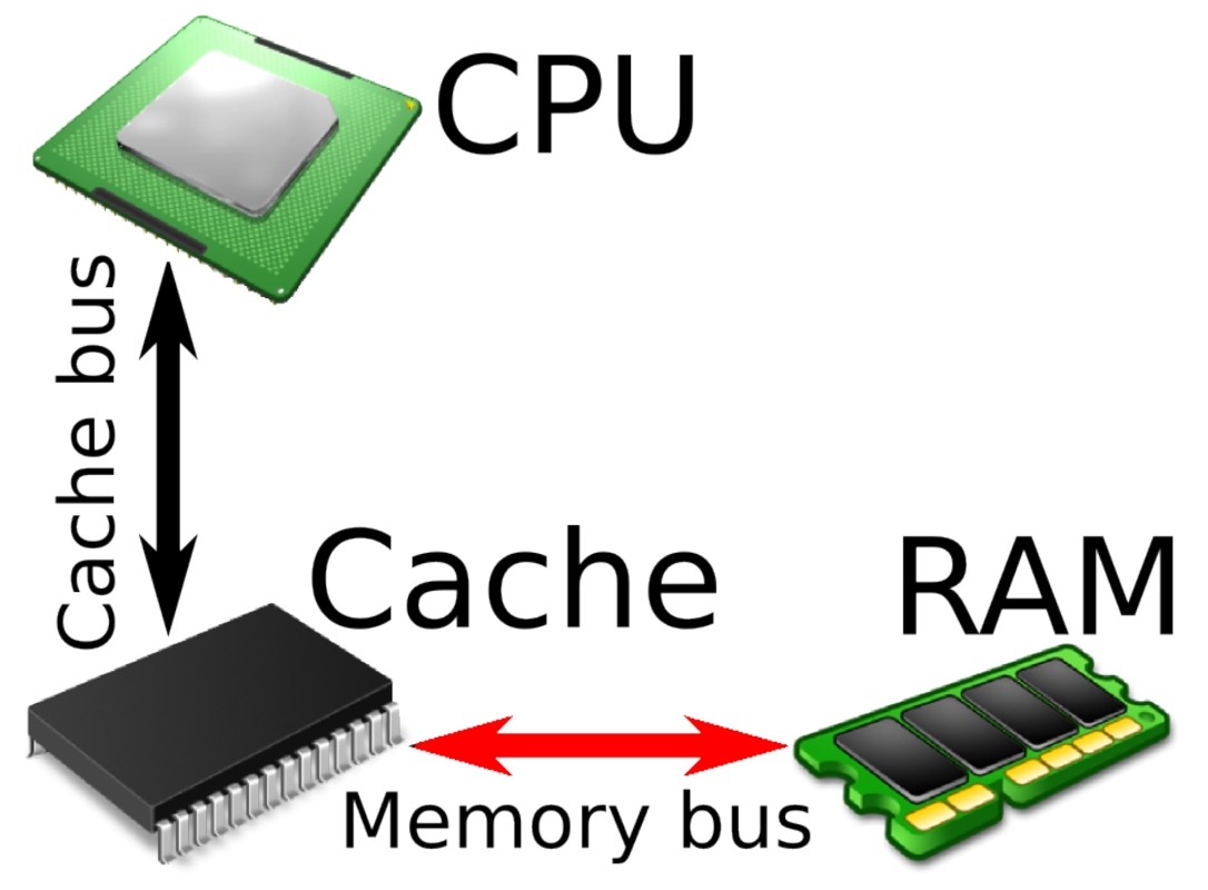
While caches are super fast, they are way too small for a typical combination of operating system + program + data, so a ‘real’ computer always has gigabytes of main memory (RAM). In a single-CPU node (M = 2..32 and N = 1), all RAM is connected to the one CPU via the caches. Every memory access that results in a cache miss will be limited by the speed of the memory bus, typically > 30 GB/s and tens of nanoseconds. So it’s immeditely obvious that for optimal performance, you should keep as much of your code and data as possible in the cache.
Single-CPU nodes are architecturally simple, but they don’t scale: the CPU can only have so many cores (currently at most 32), and it also can only address so much memory (realistically 1 TB). As much as this sounds, in HPC this is often not nearly enough.

Non-uniform memory architecture

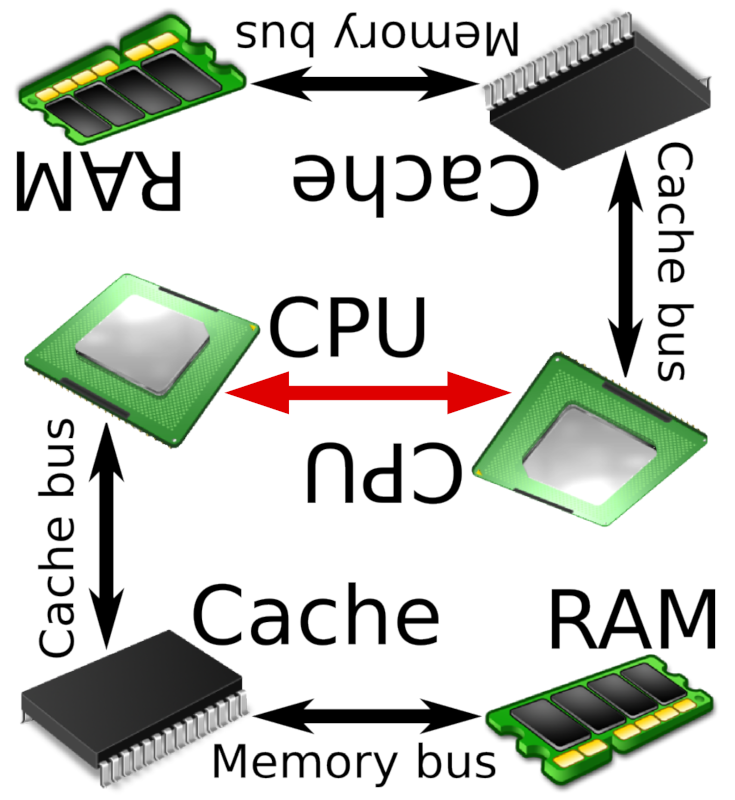
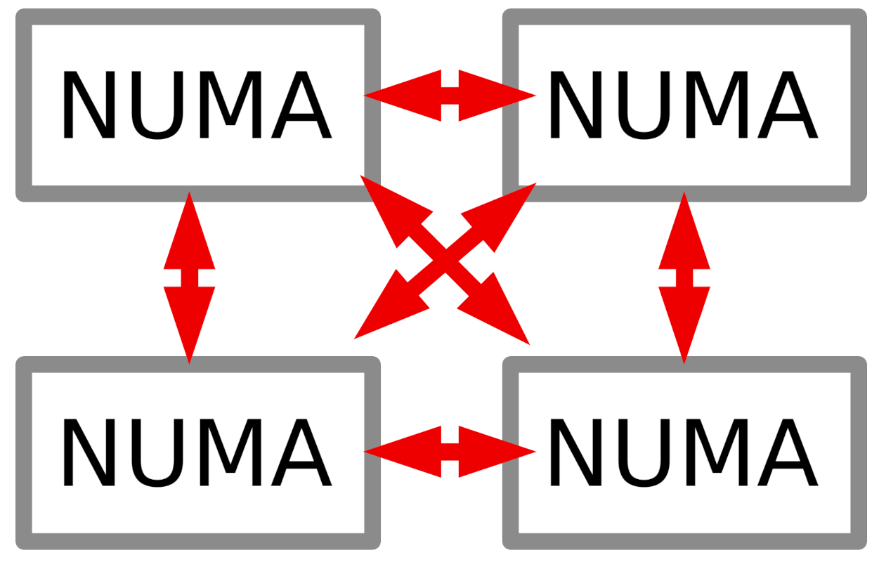
As soon as there’s more than one CPU socket in our machine (there are up to 16-way machines, so M =2..32 and N = 2..16), things get a bit more complicated: each CPU has its own memory (and caches, for that matter), but as the user of the machine, you want to be able to deal with one flat memory model that combines all RAM connected to all CPUs. This can only work in a non-uniform memory architecture (NUMA) setup, since any memory not connected to a specific CPU will only be reachable via a CPU-CPU interconnect like QuickPath/Ultra Path Interconnect (Intel) or HyperTransport/Infinity Fabric (AMD). While these interconnects are fast, they’re once again about one order of magnitude slower (as was the case from cache bus to memory bus) at around 20 GB/s bandwidth and hundreds of nanoseconds latency. On a NUMA machine, you will see all memory and all cores, but performance will be non-uniform.

This is as far as we get in “one computer”. If you need even more resources (especially RAM), you have to combine multiple nodes to form a cluster.

Cluster

A cluster introduces yet another level of interconnect: instead of CPUs like in NUMA it connects nodes via network. Another important difference is that now you’ll have to deal with multiple operating systems: one on each node (at least they’re typically all identical). Since you’re trying to keep M =2..32 cores times N = 2..16 CPUs times O = 2..10⁴ nodes busy, it’s not sufficient to just multithread, you’ll also have to multiprocess (O separate OS..) and you’ll have to employ some form of inter-process communication (IPC) across nodes unless your tasks are completely independent. Simpler and smaller clusters might use regular ethernet (1G or 10G) networking, but typically HPC clusters are built around a fast Myrinet or Infiniband network. Once again, there’s a performance penalty for scaling out onto multiple nodes: we’re now at single-digit GB/s bandwidth and microsecond latency. Two software components usually help you to get the most performance out of a cluster: a job scheduling system like TORQUE, slurm or HTCondor will take care of running submitted jobs on all available nodes, while IPC libraries like MPI and TIPC will help you to exchange efficient inter-process messages with other nodes in the cluster.

Cloud

While serious HPC almost always happens on a dedicated cluster, there are certain scientific computing workflows that use “the cloud”. For example, gene sequencing pipelines in molecular biology might be deployed on a Kubernetes cluster, which is a typical cloud setup.
“The cloud” typically differs from a real HPC cluster in 3 ways:

• usually you’ll get a bunch of virtual machines or containers that you can employ to run your jobs instead of ‘real’ hardware in a cluster

• the network is more off-the-shelf: 10G ethernet, 1 GB/s and > 10 μs

• IPC happens on a higher level: REST or SOAP interfaces instead of MPI

Now that you’ve understood the different system architectures, let’s talk about some

Implications and specialities

Keeping everything busy

As we’ve just seen, any modern computer will have a lot of cores. In fact, for the last ~ 15 years, per-core performance hasn’t really grown that much, and most speed gains in modern CPUs have come from adding ever more cores. This creates a problem for software engineering in general and HPC in particular: in many cases it’s not at all easy to keep those dozens (or in a cluster: thousands) of cores busy all the time. Of course you can run multiple instances of your code or spawn multiple threads within one process, but if these individual threads are not completely indepedent but need to exchange data, you’ll suffer from IPC penalties that scale with the square of the number of threads involved. It therefore pays off in the long run to put some thought into the layout of your code, the data structures used and how to exchange them early on.

Parallelism vs IPC costs

One aspect to keep an eye on is your level of parallelism: the smaller your individual thread is, the easier it’ll be to keep all cores on all nodes occupied as you’ll have more threads to work with. IPC costs however will be higher since more communication partners are involved. You might have to experiment to find the best granularity for your system.

SIMD

SIMD stands for single instruction, multiple data and means that you’re performing an operation not just on one variable, but a whole set of them. Typical examples are vector or matrix operations. If your code executes a lot of those, you might benefit greatly from

GPGPU

General-purpose graphics processing units denote graphics cards being used for general computation. Graphics cards owe their impressive 3D performance to their vast number (thousands) of execution units that can run a limited set of instructions extremely fast. If the calculations in your code can be mapped onto this model, you can profit from impressive speed gains (100x fold or more). GPGPU is not applicable to all scientific computing problems and has downsides too (e.g. limited onboard memory, limited instruction set), but it’s definitely something to keep in mind and play around with. There’s NVIDIA’s powerful CUDA framework and the more general OpenCL to get you started.

AVX

In recent years, also CPUs (both Intel and AMD) have gained SIMD capabilities: AVX (Advanced Vector Extensions). You’ll have to consult your compiler documentation for the corresponding compile flags.

Storage

We’ve talked a lot about CPUs, memory, threads and so on, but now it’s time to address another part in every scientific computing system: storage. After all, what good are all your beautiful results if you have nowhere to store them? Typically you’ll find two types of storage:

Local storage

Local storage is directly built into your PC or node in the form of hard drives or SSDs. It’s usually only meant to be used on this very machine, even though it might be shared in some cases. It’s typically referred to as scratch and is supposed to be used as a temporary place for your data while the calculation is ongoing - often, there’s no backup for scratch. In most cases, it’s not very large (GB to a few TB), but pretty fast (esp. for SSDs).

Network storage

Additionally you’ll usually find a much larger, permanent storage space mounted over the network. This is accessible from all nodes, there’s backup, but it comes at a cost: since it’s a network file system (NFS or a cluster file system), it’s usually slower than local scratch. As soon as your data has reached any semi-permanent state, it should probably go onto network storage.

Storage as a bottleneck

While it is true that it might be possible to simply generate too much data (especially in simulations, often by mistake..), in most cases storage capacity will not be a major limit to your scientific computing endeavours - storage is well understood and it’s not too difficult to have enough of it. The same is not true for IOPS however. It’s trivially possible for one process to saturate the I/O capabilities of a given machine, no matter how fast. This is especially true for network storage, but even local HDD storage can only handle so many IOPS. In the worst case, your code will bring the whole I/O subsystem of the machine to a halt, effectively rendering it unusable for you and everybody else. The I/O cascade of hell goes something like this:

everybody happy < sequential read OR write < sequential read+write < random read OR write < random read+write < random read+write from many threads < machine kaput

Sequential means that you’re reading or writing chunks of reasonable size (hundreds of kB to a few MB) at a time while random I/O wildly jumps around in a file and reads/writes very small amounts of data. Random I/O creates a high number of IOPS which will kill any storage subsystem, especially if it’s HDD based.

So in order to get the best performance out of your code and not render the hardware unusable for everyone else, you should make sure to

• always run your calculations on local scratch, then copy the results to network storage when finished

• open as few files as possible and keep them open as long as possible

• read and or write contiguous chunks of data instead of jumping around in those files

Limits revisited

With all this in mind, it’s time to come back to our original question “Can you partition the problem into N independent smaller tasks?” in order to identify the probable bottleneck for your problem and get an idea of how well it will scale.

Yes, independent tasks

As we’ve seen before when we talked about bus speeds, in this case the follow-up question is: “Does each task (code + data) fit into the L1-L3 caches?”. If this is true, your performance will likely be limited by the raw processing power (”CPU bound”). A CPU with faster cores (often: more GHz) would make things faster. If false, your bottleneck might turn out to be the memory bus (”memory bound”). If you can’t optimize your problem to fit (better) into the cache(s), faster memory could help (but the speedup is quite limited here).

In both these situations, your overall performance across many cores on many nodes will probably scale linearly with the number of cores involved (line 1 in the graph above). Due to all sorts of ‘losses’ (scheduling, network file systems..) your gradient might not reach 1, but adding more cores will give you more performance.

No, I have communication between my tasks

As discussed previously, if your tasks need to communicate, you’ll encounter IPC performance penalties, and your bottleneck will be the communication overhead and the interconnect (at least for larger numbers of cores). The overall performance of your system will most likely scale like line 2 in the graph: for a certain number of cores your performance gain will saturate, and might turn negative if going even further.

The software side

In the previous chapters we’ve learned how the underlying hardware architecture will influence your code’s performance. Now let’s turn to the software side of things. First:

Programming languages

There’s an almost innumerable variety of programming languages out there, and most of them can be (and probably have been) used for scientific computing. Some have been around for more than 60 years (Fortran) while others are pretty new (Julia). They all have their strengths, weaknesses and specialties, and the choice of programming language (and the accompanying libraries) will influence the progress of your project in at least two ways: development time and final performance. In some cases you simply won’t have a say in the choice of the language to be used, but if you do, it’s important to know what to look out for. Here are some guidelines:

What may you use?

• not everything might be available on the target machine

• there might be libraries or existing code you want or have to use

• you might need to collaborate with others

What should you use?

• which language would be the fastest in terms of

  • development time

  • execution speed

• have (parts of) your problems already been solved in some code or library in one language or other?

What can you use?

• Which language(s) are you familiar with?

• How fast can you learn (and master) another one?

Compiled vs interpreted languages

Above all other dichotomies (statically vs dynamically typed, procedural vs functional, object oriented vs structured) the one between a compiled and an interpreted language will probably have the largest impact on your scientific computing project.

Interpreter languages

Interpreter languages (also called scripting languages, examples include Python, PHP, Perl..) originally used the following workflow: each time you ‘run’ such a program, the operating system starts the appropriate interpreter which executes your script line by line. No executable file will be created on disk. This allows for ‘rapid prototyping’ programming since you can immediately test each small change in the program. Downside: execution isn’t very fast, since the interpreter is basically going through the problem step by step. In a nutshell: “fast coding, slow code”.

Compiler languages

Classic compiled languages like C/C++, Rust, Fortran, Go etc require a dedicated compile run each time you’ve changed your code and want to test it. The compiler compiles and links the code and generates an executable file on disk that you can start. Compared to interpreter languages, this requires an additional step before you see the result of your code changes. On the upside, the compiler has a lot more possibilities to optimize execution, so compiled programs usually run faster: “slow coding, fast code”.

In recent years interpreter languages have changed a lot and nowadays usually don’t get interpreted line by line, but are compiled on the fly into an intermediate bytecode that also offers most of the performance benefits of a compiled language. Furthermore, some compiler languages (most obvious example: Java) also compile into bytecode, so the gap between compiled and interpreted languages is getting narrower. The latter still have the advantage of easier handling and faster turnaround though.

Optimizations

Aside from picking the “right” language for the job, there are a lot of other factors that can dramatically increase the performance of your code. Here are some ideas:

• pick the right compiler (gcc, llvm, Intel, PGI..) and the compile flags best matching your problem. This can easily yield a factor of 2 or even more

• use optimized libraries (BLAS, LAPACK, BOOST, NumPy..). For most interpreter languages you’ll find bindings or wrappers for those highly optimized C libraries that speed up HPC tasks tremendously.

• use data types that reflect your problem (e.g. bit fields for Ising spin glasses, single vs double precision floats…)

• think about cache + memory alignment and locality

• use a profiler to identify code hot spots

• if you have access to the hardware and OS, both can be tuned for specific workloads

• individual threads can be pinned to specific cores

• pick sensible file formats (HDF, packed binary, XML, CSV…)

• think about what you need to write to disk, how often, how many files

Tips, hints and anecdotes

We’ll end this module with a small collection of tips and real-life stories from ISG’s stock of experience.

• use checkpointing to prevent data loss in case of a crash, power outage or network problem.

• good random numbers are surprisingly hard to generate - especially if you need lots of them.

• use job queuing systems if available. It’ll make your and other people’s lives easier.

• never ever swap, ever! Disks are so much slower than memory that you’ll completely kill your performance. The situation is a bit better for SSDs, but you should still avoid it if you can.

• once again: make sure you’re using all available cores.

• if you have to use network storage for long-running jobs (even though you really shouldn’t), be aware of network interruptions.

• on ISG’s behalf: please don’t move / rename a 10T folder without telling us. It’ll create headaches for our backup system.

• on ISG’s behalf: do not create millions of small files on the file server. This will waste a lot of space and kill performance. Create tgz or zip archives instead.

Web content

There is a nice interactive Pluto notebook that lets you explore many of the topics of this module.

Glossary

Abbreviation	Explanation
CPU	Central Processing Unit → the physical processor in a computer
Core	individual execution unit within a CPU
Process	one ‘program’ running on a computer
Thread	sequence of instructions that may execute in parallel with others, within one process
Cache	small + fast memory in or close to CPU
Interconnect	data bus between two units
Throughput	amount of data transferred per time unit
Latency	packet delay time
GPGPU	General-purpose graphics processing unit, use graphics cards for computation
NUMA	non-uniform memory access, one way of building multi-CPU computers
IPC	inter-process communication
IOPS	I/O operations per second